Queuing theory basics part 2: multiple servers

These are my notes for the following three lectures on queueing theory:

• Part 1 - notes for Lec-30 Queueing Models
• Part 1 - notes for Lec-31 Single Server Queueing Models
• Part 2 - notes for Lec-32 Multiple Server Queueing Models

Multiple servers, infinite queue (M/M/c)

Consider the case with $c$ servers and infinite queue capacity. Assume people form a common line and are served by the first available server. Additionally, assume all servers have identical service rate $\mu$.

The effective service rate depends on the number of people in the system. If there are $n \le c$ people are in the system, then the service rate is $n \mu$. If there are $n \ge c$ people in the system, then all servers are busy, so the service rate is $c \mu$.

Distribution of queue lengths

We can now compute a recurrence similar to the single server case:

$$\begin{aligned} p_n(t+h) &=\; P(\text{1 arrival, 0 service}) \cdot p_{n-1}(t)\\ &\;+ P(\text{0 arrival, 1 service}) \cdot p_{n+1}(t)\\ &\;+ P(\text{0 arrival, 0 service}) \cdot p_n(t)\\ &=\; \lambda h \cdot (1 - \mu_{n-1} h) \cdot p_{n-1}(t)\\ &\;+ (1 - \lambda h) \cdot \mu_{n+1} h \cdot p_{n+1}(t)\\ &\;+ (1 - \lambda h) \cdot (1 - \mu_n h) \cdot p_n(t)\\ &\approx \lambda h p_{n-1}(t) + \mu_{n+1} h p_{n+1}(t) + (1 - \lambda h - \mu_n h) p_n(t)\\ \implies \frac{p_n(t+h) - p_n(t)}{h} &= \lambda p_{n-1}(t) + \mu_{n+1} p_{n+1}(t) - (\lambda + \mu_n) p_n(t). \end{aligned}$$

At steady-state, the distribution is time-independent, so $\frac{p_n(t+h) - p_n(t)}{h} = 0$. Thus

$$\lambda p_n{n+1} + \mu_{n+1} p_{n+1} = (\lambda + \mu_n) p_n.$$

Similarly, we find $\mu_1 p_1 = \lambda p_0$ (or $p_1 = \frac{\lambda}{\mu_1} p_0$). Now

$$\begin{aligned} \lambda p_0 + \mu_2 p_2 = (\lambda + \mu_1) p_1 = \lambda p_1 + \mu_1 p_1 = \lambda p_1 + \lambda p_0\\ \implies \mu_2 p_2 = \lambda p_1 \implies p_2 = \frac{\lambda}{\mu_2} p_1. \end{aligned}$$

The recurrence continues similarly:

$$p_n = \frac{\lambda^n}{\prod_{i=1}^n \mu_i} p_0 = \begin{cases} \frac{\rho^n}{n!} p_0 &\text{ if } n \le c\\ \frac{\rho^n}{c! c^{n-c}} p_0 &\text{ if } n \ge c \end{cases}.$$

Now we can compute $p_0$:

$$\begin{aligned} 1 = \sum_{n \ge 0} p_n = \sum_{n=0}^{c-1} \frac{\rho^n}{n!} p_0 + \sum_{n \ge c} \frac{\rho^n}{c!c^{n-c}} p_0 = p_0 \left( \sum_{n=0}^{c-1} \frac{\rho^n}{n!} + \frac{\rho^c}{c!} \frac{1}{1-\rho/c} \right)\\ \implies p_0 = \left( \sum_{n=0}^{c-1} \frac{\rho^n}{n!} + \frac{\rho^c}{c!} \frac{1}{1-\rho/c} \right)^{-1}. \end{aligned}$$

Expected queue length and wait time

There are only people waiting if there are $n \ge c$ people in the system, so the expected number of people waiting is

$$\begin{aligned} L_q &= \sum_{n \ge c} (n-c) p_n = \sum_{n \ge 0} n p_{n+c} = \sum_{n \ge 1} n \frac{\rho^{n+c}}{c! c^n} p_0\\ &= \frac{p_0 \rho^{c+1}}{c! c} \sum_{n \ge 1} n \frac{\rho^{n-1}}{c^{n-1}}\\ &= \frac{p_0 \rho^{c+1}}{c! c} \frac{\mathrm{d}}{\mathrm{d} (\rho/c)} \sum_{n \ge 1} \frac{\rho^n}{c^n}\\ &= \frac{p_0 \rho^{c+1}}{c! c} \frac{\mathrm{d}}{\mathrm{d} (\rho/c)} \left(\frac{1}{1-\rho/c} - 1\right)\\ &= \frac{p_0 \rho^{c+1}}{c! c} \left( \frac{1}{(1-\rho/c)^2} \right)\\ &= \frac{p_0 \rho^{c+1}}{(c-1)!(c-\rho)^2}. \end{aligned}$$

A similar calculation can be carried out for the expected number of people in the system, $L_s = L_q + \rho$. With these, can can again calculate the expected wait time and service time using Little's law:

$$L_q = \lambda W_q, \qquad L_s = \lambda W_s.$$

In the case of multiple servers, the calculation of utilization is more complicated. It can be thought of as the average probability that any one server is busy, assuming people are uniformly distributed across servers. That is,

$$U = \sum_{n=0}^{c-1} \frac{n}{c} p_n + \sum_{n \ge c} p_n = \frac{\rho}{c}.$$

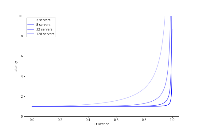
As before, we can plot the latency with respect to utilization:

import matplotlib.pyplot as plt
import numpy as np
from scipy.special import factorial

def plot_latency(c, **kwargs):
   rho = np.linspace(0, c, 1000)
   p0 = 1/(sum(rho**n/factorial(n) for n in range(0, c)) +
           rho**c/factorial(c)/(1-rho/c))
   utilization = rho/c
   latency = p0*rho**c/(factorial(c-1)*(c-rho)**2) + 1
   plt.plot(utilization, latency, label=f'{c} servers', **kwargs)

plt.figure(figsize=(9, 6))
plt.ylim(0, 10)
plt.xlabel('utilization')
plt.ylabel('latency')
for c, alpha in [(2, 0.25), (8, 0.5), (32, 0.75), (128, 1.0)]:
   plot_latency(c, alpha=alpha, color='blue')
plt.legend()
plt.savefig('mmc-latency.png')
plt.show()

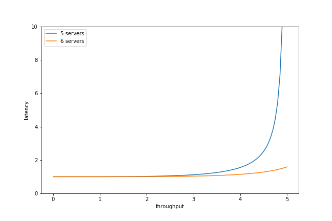
We can also plot the latency with respect to the arrival rate, holding the service rate fixed. So long as $\lambda \le c \mu$, the arrival rate is equal to the throughput of the system (if $\lambda > c \mu$, the queue will grow indefinitely). This demonstrates that adding more servers reduces the latency:

import matplotlib.pyplot as plt
import numpy as np
from scipy.special import factorial

rho = np.linspace(0, 5, 100)
def plot_latency(c, **kwargs):
   p0 = 1/(sum(rho**n/factorial(n) for n in range(0, c)) +
           rho**c/factorial(c)/(1-rho/c))
   latency = p0*rho**c/(factorial(c-1)*(c-rho)**2) + 1
   plt.plot(rho, latency, label=f'{c} servers', **kwargs)

plt.figure(figsize=(9, 6))
plt.ylim(0, 10)
plt.xlabel('throughput')
plt.ylabel('latency')
plot_latency(5)
plot_latency(6)
plt.legend()
plt.savefig('mmc-throughput.png')
plt.show()

Multiple servers, finite queue (M/M/c/N)

Consider a finite queue of capacity $N$ feeding into $c$ servers, where people arrive at rate $\lambda$ and each server has rate $\mu$. In the following, assume $N > c$.

Distribution of queue lengths

The recurrence for the distribution over the number of people in the system is the same as the M/M/1/N queue:

$$p_n = \begin{cases} \frac{\rho^n}{n!} p_0 &\text{ if } n \le c\\ \frac{\rho^n}{c!c^{n-c}} p_0 &\text{ if } n \ge c \end{cases}.$$

We can now compute the probability that there are 0 people in the system:

$$\begin{aligned} 1 = \sum_{n=0}^N p_n &= \sum_{n=0}^{c-1} \frac{\rho^n}{n!} + \sum_{n=c}^N \frac{\rho^n}{c!c^{n-c}} p_0\\ &= p_0 \left( \sum_{n=0}^{c-1} \frac{\rho^n}{n!} + \frac{\rho^c}{c!} \cdot \frac{1 - (\rho/c)^{N-c+1}}{1 - \rho/c} \right)\\ \implies p_0 &= \left( \sum_{n=0}^{c-1} \frac{\rho^n}{n!} + \frac{\rho^c}{c!} \cdot \frac{1 - (\rho/c)^{N-c+1}}{1 - \rho/c} \right)^{-1}. \end{aligned}$$

Expected queue length and wait times

We can compute the expected queue length similar to the M/M/c case:

$$\begin{aligned} L_q &= \sum_{n=c}^N (n-c) p_n = \sum_{n=0}^{N-c} n p_{n+c} = \sum_{n=0}^{N-c} n \frac{\rho^{n+c}}{c!c^n} p_0\\ &= \frac{\rho^{c+1} p_0}{(c-1)!} \cdot \frac{1 - (\rho/c)^{N-c+1} - (N-c+1)(1-\rho/c)(\rho/c)^{N-c}}{(c-\rho)^2}. \end{aligned}$$

And the expected number of people in the system:

$$\begin{aligned} L_s &= \sum_{n=0}^N n p_n\\ &= p_0 \rho \sum_{n=0}^{c-2} \frac{\rho^n}{n!} + \frac{p_0 \rho^c}{c!} \bigg( c \frac{1 - (\rho/c)^{N-c+1}}{1-\rho/c}\\ &\qquad+ \frac{\rho}{c} \frac{1 - (\rho/c)^{N-c+1} - (N-c+1)(1-\rho/c)(\rho/c)^{N-c}}{(1-\rho/c)^2} \bigg). \end{aligned}$$

The probability that the queue is full and thus someone is rejected is $p_N = \frac{\rho^N}{c!c^{N-c}} p_0$. As with the M/M/1/N queue, there is an effective arrival rate $\lambda_\text{eff} = \lambda (1-p_N)$, from which we can derive the service and wait times $W_s = L_s/\lambda_\text{eff}$ and $W_q = L_q/\lambda_\text{eff}$.

Simulation

Here is a Jupyter notebook simulating a single- and multiple-server infinite queue:

• HTML
• Notebook