Queuing theory basics part 1: single server

These are my notes for the following three lectures on queueing theory:

• Part 1 - notes for Lec-30 Queueing Models
• Part 1 - notes for Lec-31 Single Server Queueing Models
• Part 2 - notes for Lec-32 Multiple Server Queueing Models

In a queueing model, people arrive at the queue, wait in line, and then are serviced by a server. There may be a single server or multiple servers (sharing a single line). The queue capacity may be finite or infinite. In a finite queue, people may be unable to join the queue if it is full.

Arrivals and servers are each modeled by a distribution over their rates.

• Arrivals are typically modeled by a Poisson distribution with rate $\lambda$ (e.g., 4 per hour).
• Service times are typically modeled by an exponential distribution with rate $\mu$ (e.g., 5 per hour). The mean service time is then $\frac{1}{\mu}$.

In the following, we will assume that arrivals and servers follow a Poisson and exponential distribution, respectively. These two distributions are memoryless, meaning that arrivals are independent of one another, as are service times. Note that if we have an infinite queue capacity and $\lambda > \mu$, then the queue will grow indefinitely.

The queueing discipline determines which person in line gets serviced next. An example queueing discipline is first-in, first-out (FIFO), where people are serviced in the order in which they arrive. Steady-state behavior is often the same regardless of queueing discipline. In the following, we will assume a FIFO queueing discipline.

Notation

Queues can be specified in Kendall's notation. The notation is A/S/c/K/N/D, where

• A = arrival process, with "M" denoting a memoryless process.
• S = service time distribution, with "M" denoting a memoryless distribution of service time.
• c = number of servers
• K = queue capacity
• N = population size (total population from which arrivals are drawn)
• D = queueing discipline, e.g., FIFO

For example, a M/M/1/∞/∞/FIFO queue is a memoryless queue with 1 server, infinite queue capacity, infinite population, and FIFO queueing discipline. If unspecified, we assume K/N/D is ∞/∞/FIFO. For example, M/M/1 = M/M/1/∞/∞/FIFO.

Single server, infinite queue (M/M/1)

Let's consider the case of a queue with infinite capacity and a single server. Assume that arrivals are Poisson distributed with rate $\lambda$ and service times are exponentially distributed with rate $\mu$.

Distribution of queue lengths

In a Poisson distribution, no two events occur at the same instant. Let $h$ be an infinitesimal interval in which exactly 0 or 1 event occurs.

Let $p_n(t)$ to be the probability that $n$ people are in the system (waiting in line or being serviced) at time $t$. Then

$$\begin{aligned} p_n(t+h) =\; &P(\text{1 arrival, 0 service}) \cdot p_{n-1}(t)\\ + &P(\text{0 arrival, 1 service}) \cdot p_{n+1}(t)\\ + &P(\text{0 arrival, 0 service}) \cdot p_n(t). \end{aligned}$$

As $h$ is defined to be the interval in which at most 1 event occurs, there is no $P(\text{1 arrival, 1 service}) \cdot p_n(t)$ term.

In a Poisson distribution, the probability of $k$ events occurring in an interval $\tau$ is

$$P(k \text{ events in interval } \tau) = f(k; \tau) = e^{\lambda \tau} \frac{(\lambda \tau)^k}{k!}.$$

This distribution has mean $E[k] = \sum_{k \ge 0} k f(k; \tau) = \lambda \tau$. As we have defined $h$ to be an interval with at most 1 event,

$$P(1 \text{ event}) = 0 \cdot P(0 \text{ events}) + 1 \cdot P(1 \text{ event}) = E_{f(k; h)}[k] = \lambda h$$

Therefore

$$\begin{aligned} p_n(t+h) =\; &\lambda h \cdot (1 - \mu h) \cdot p_{n-1}(t)\\ + &(1 - \lambda h) \cdot \mu h \cdot p_{n+1}(t)\\ + &(1 - \lambda h) \cdot (1 - \mu h) \cdot p_n(t). \end{aligned}$$

To first order in h,

$$p_n(t+h) \approx \lambda h p_{n-1}(t) + \mu h p_{n+1}(t) + (1 - \lambda h - \mu h) p_n(t),$$

thus

$$\frac{p_n(t+h) - p_n(t)}{h} = \lambda p_{n-1}(t) + \mu p_{n+1}(t) - (\lambda + \mu) p_n(t).$$

At steady state, we expect a unchanging distribution of queue lengths, so

$$0 = \frac{p_n(t+h) - p_n(t)}{h} \implies \lambda p_{n-1} + \mu p_{n+1} = (\lambda + \mu) p_n. \qquad{(1)}$$

When the queue is empty, no service occurs ( $P(\text{0 service}) = 1$), so

$$\begin{aligned} p_0(t+h) &= P(\text{0 arrivals, 1 service}) \cdot p_1(t) + P(\text{0 arrivals, 0 service}) \cdot p_0(t)\\ &= (1 - \lambda h) \cdot \mu h \cdot p_1(t) + (1 - \lambda h) \cdot 1 \cdot p_0(t)\\ &\approx \mu h \cdot p_1(t) + (1 - \lambda h) p_0(t). \end{aligned}$$

Hence, at steady state,

$$0 = \frac{p_0(t+h) - p_0(t)}{h} = \mu p_1(t) - \lambda p_0(t) \implies \mu p_1 = \lambda p_0. \qquad{(2)}$$

By (1) ( $n=1$ ) and (2),

$$\begin{aligned} &\lambda p_0 + \mu p_2 = (\lambda + \mu) p_1 = \lambda p_1 + \mu p_1 = \lambda p_1 + \lambda p_0\\ &\implies p_2 = \frac{\lambda}{\mu} p_1 = \left(\frac{\lambda}{\mu}\right)^2 p_0. \end{aligned}$$

Let $\rho = \frac{\lambda}{\mu}$. By a similar argument, $p_n = \rho^n p_0$ for all $n \ge 1$. As this is a probability distribution,

$$1 = \sum_{n \ge 0} p_n = p_0 \sum_{n \ge 0} \rho^n = p_0 \cdot \frac{1}{1-\rho} \implies p_0 = 1 - \rho.$$

Therefore

$$p_n = \rho^n p_0 = \rho^n (1 - \rho). \qquad{(3)}$$

Expected queue length and wait time

Using the distribution of the number of people in the system (3), we can derive the expected number of people in the system (recall that $\rho = \frac{\lambda}{\mu}$):

$$\begin{aligned} L_s = E_p[n] &= \sum_{n \ge 0} n \rho^n (1-\rho)\\ &= (1-\rho) \rho \sum_{n \ge 1} n \rho^{n-1}\\ &= (1-\rho) \rho \frac{\mathrm{d}}{\mathrm{d}\rho} \sum_{n \ge 1} \rho^n = (1-\rho) \rho \frac{\mathrm{d}}{\mathrm{d}\rho} \frac{1}{1-\rho}\\ &= (1-\rho) \rho \frac{1}{(1-\rho)^2} = \frac{\rho}{1-\rho}. \end{aligned}$$

The expected number of people being serviced is the expected proportion of time the system is nonempty, i.e., $1 - p_0 = 1 - (1-\rho) = \rho$. Thus the expected number of people waiting to be serviced is $L_q = L_s - \rho$.

The expected time spent in the system (including time being serviced) is related to the queue length by Little's law: $L_s = \lambda W_s$. A similar relation applies to the expected time spent waiting to be serviced: $L_q = \lambda W_q$.

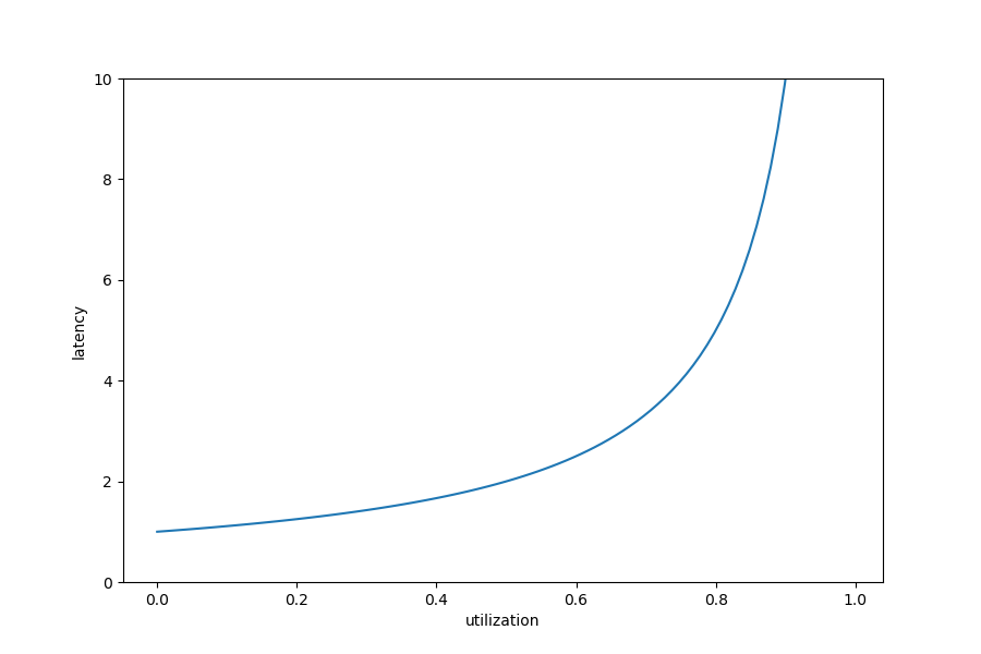
The utilization is the probability that the server is busy:

$$U = 1 - p_0 = 1 - (1 - \rho) = \rho.$$

If we plot the service time (i.e., latency) with respect to utilization, we see that it begins increasing rapidly around $U=0.8$:

import matplotlib.pyplot as plt
import numpy as np

rho = np.linspace(0, 1, 100)
latency = 1/(1-rho)

plt.figure(figsize=(9, 6))
plt.ylim(0, 10)
plt.xlabel('utilization')
plt.ylabel('latency')
plt.plot(rho, latency)
plt.savefig('mm1-latency.png')
plt.show()

Single server, finite queue (M/M/1/N)

The recurrence for $p_n = \rho^n p_0, n \le N$ remains the same, and we can use it to compute $p_0$:

$$\begin{aligned} 1 = \sum_{n=0}^N p_n = \sum_{n=0}^N \rho^n p_0 = p_0 \cdot \frac{1-\rho^{N+1}}{1-\rho}\\ \implies p_0 = \frac{1-\rho}{1-\rho^{N+1}}. \end{aligned}$$

With this, we can compute the expected number of people in the system:

$$\begin{aligned} L_s &= \sum_{n=0}^N n p_n = \sum_{n=0}^N n \rho^n p_0 = p_0 \rho \sum_{n=0}^N n \rho^{n-1} = p_0 \rho \frac{\mathrm{d}}{\mathrm{d}\rho} \sum_{n=0}^N \rho^n\\ &= p_0 \rho \frac{\mathrm{d}}{\mathrm{d}\rho} \frac{1-\rho^{N+1}}{1-\rho} = p_0 \rho \cdot \frac{1 + N \rho^{N+1} - (N+1) \rho}{(1-\rho)^2}. \end{aligned}$$

A similar calculation may be performed for $L_q$, or we can reason through it as follows: As people are unable to join the queue when it is full, there is an effective arrival rate $\lambda_\text{eff} < \lambda$. A person may only join the queue if there are fewer than $N$ others in the system, which happens with probability $1-p_N$. Thus $\lambda_\text{eff} = \lambda (1 - p_N)$. From this, we can compute the expected queue length, service time, and wait time:

$$L_q = L_s - \frac{\lambda_\text{eff}}{\mu}, \qquad W_s = \frac{L_s}{\lambda_\text{eff}}, \qquad W_q = \frac{L_q}{\lambda_\text{eff}}.$$

Continued in part 2...