Reconstructing audio from its spectrogram

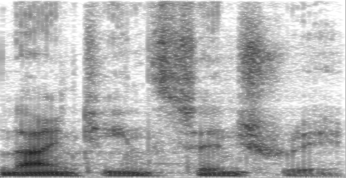
Spectrogram of a person saying — Derived from spectrogram by Wikipedia user Aquegg, public domain.

A spectrogram is a visualization of the frequencies present in audio. Time is shown on the x-axis and frequency is shown on the y-axis. The above spectrogram is from the Wikipedia article Spectrogram and was generated from audio of someone speaking the words "nineteenth century".

The discrete Fourier transform

Let $x$ be a signal whose value is sampled at a rate $R$ (e.g., 44100 samples/second). Let $x[n]$ denote the $n^\text{th}$ sample, i.e., the value of the signal at time $n/R$ .

The discrete Fourier transform (DFT) takes a signal and calculates which frequencies are present in it. For example, if $x$ were the sum of a sine wave with frequency 500 Hz and another with frequency 600 Hz, then the DFT would have peaks at 500 Hz and 600 Hz. More precisely, if $X = \operatorname{DFT}(x)$ , then $X[k]$ is the coefficient of the sinusoid with frequency $kR/N$ in the original signal, where $N$ is the total number of samples. Note that $X[k]$ is a complex number. The DFT is typically calculated with an algorithm called the fast Fourier transform (FFT).

Window functions and the short-time Fourier transform

A window function is a function that is multiplied against a signal elementwise to "focus" on a small part of the signal and ignore the rest:

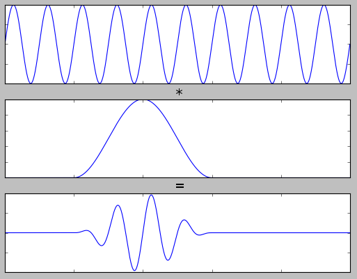
The window function is the one in the middle. This one is the Hann window.

The short-time Fourier transform (STFT) is the DFT calculated over many small windows of the signal. More precisely, $\operatorname{STFT}(x)[m,k] = \operatorname{DFT}(x_m * w)[k],$ where $*$ denotes elementwise multiplication and $x_m$ is the signal shifted over by $m$ places ( $x_m[n] = x[m+n]$ ).

Let's break that down: The elementwise multiplication $x_m * w$ zeros out all but a small part of the signal starting at position $m$ . Then we apply the DFT and extract the $k^\text{th}$ element, i.e., the coefficient associated with frequency $kR/N$ . Putting that back together, $\operatorname{DFT}(x_m * w)[k]$ is the magnitude of frequency $kR/N$ starting at time $m/R$ in the original signal.

A spectrogram is the square of the STFT: $\operatorname{spec}(x)[m,k] = |\operatorname{STFT}(x)[m,k]|^2.$ Typically the spectrogram isn't computed at every value of $m$ , but instead on wider-spaced, overlapping windows.

Inverting the spectrogram

The DFT comes with a counterpart to undo the transformation, the inverse discrete Fourier transform (IDFT). It has the property that $\operatorname{IDFT}(\operatorname{DFT}(x)) = x$ .

Suppose we have computed the STFT to be $X = \operatorname{STFT}(x)$ . We can then compute the inverse short-time Fourier transform (ISTFT) by $\operatorname{ISTFT}(X) = \sum_m \operatorname{IDFT(X[m,\cdot])},$ where " $\cdot$ " denotes an entire row of the array. This assumes that overlapping window functions always sum to 1, which can be achieved through normalization. The ISTFT has the property that $\operatorname{ISTFT}(\operatorname{STFT}(x)) = x$ .

Now suppose we are given a spectrogram $S = \operatorname{spec}(x)$ . The spectrogram throws away some information relative to the STFT: by squaring each element, we lose the phase, the amount by which each sine wave is shifted horizontally. If we were to invert the spectrogram by simply taking its ISTFT, it would be unintelligible because the phases would be incorrect.

Thankfully, there is an iterative algorithm due to Griffin and Lim (1984) to estimate the phase: $\begin{aligned} x_0 &= \operatorname{ISTFT(S)};\\ X_{i+1} &= \operatorname{ISTFT}\left( S \cdot \frac{\operatorname{STFT}(x_i)}{|\operatorname{STFT}(x_i)|} \right). \end{aligned}$ After a few iterations, this yields a decent approximation of the original signal ( $x_{10} \approx x$ ).

Implementation

The following implementation is written in Python 3.10.1 and uses NumPy 1.21.5, SciPy 1.7.3, and Pillow 9.0.0.

# To install dependencies:
#   python3 -m venv venv
#   source venv/bin/activate
#   pip install numpy==1.21.5 scipy==1.7.3 Pillow==9.0.0

from PIL import Image
import numpy as np
from scipy.signal.windows import hann
from scipy.io import wavfile

The STFT and ISTFT are defined as before. Since audio signal are real-valued, we can use NumPy's rfft and irfft functions, which compute the DFT and IDFT for real-valued signals.

def rstft(x, win, hop):
    """
    Compute the short-time Fourier transform (STFT) of a real-valued signal.

    Parameters
    ----------
    x : array_like
        Signal to compute the STFT of.
    win : int
        Width of the Hann window.
    hop : int
        Number of samples to skip between windows. If `hop < win`, the windows
        will overlap. Normalization to compensate for window overlap is
        performed automatically.

    Returns
    -------
    y : array_like
        STFT of `x`. Axis 0 is frequency and axis 1 is time.
    """
    # The Hann window has the property that at 50% overlap, overlapping windows
    # sum to 1. For denser overlaps, we compute a scaling factor.
    w = hann(win)
    scale = 2 * hop/win

    # Round length up to the nearest multiple of `hop`.
    length = ((x.shape[0] - win - 1) // hop + 1) * hop + win
    x_pad = np.array(x)
    x_pad.resize(length)

    # Compute the STFT.
    y = []
    for t in range(0, length - win + hop, hop):
        y.append(np.fft.rfft(x_pad[t:t+win] * w))
    return scale * np.array(y).T

def irstft(y, win, hop):
    """
    Compute the inverse short-time Fourier transform (ISTFT) of a real-valued
    signal.

    Parameters
    ----------
    y : array_like
        STFT to calculate the ISTFT of. Axis 0 is frequency and axis 1 is time.
    win : int
        Width of the Hann window.
    hop : int
        Number of samples to skip between windows. If `hop < win`, the windows
        will overlap.

    Returns
    -------
    x : array_like
        ISTFT of `y`.
    """
    length = win + hop * (y.shape[1] - 1)
    x = np.zeros((length,))
    for t in range(y.shape[1]):
        x[t*hop:t*hop+win] += np.fft.irfft(y[:,t])
    return x

Now Griffin and Lim's algorithm:

def reconstruct(y, iterations, win, hop):
    """
    Reconstruct a signal from its spectrogram.

    Parameters
    ----------
    y : array_like
        Spectrogram. Linear scale, not log scale. Axis 0 is frequency and
        axis 1 is time.
    iterations : int
        Number of iterations to run the algorithm. More iterations produces a
        better reconstruction.
    win : int
        Width of the Hann window.
    hop : int
        Number of samples to skip between windows. If `hop < win`, the windows
        will overlap.

    Returns
    -------
    x : array_like
        Reconstructed signal.

    References
    ----------
    (1) Griffin, D.; Lim, J. Signal Estimation from Modified Short-Time Fourier
    Transform. IEEE Transactions on Acoustics, Speech, and Signal Processing
    1984, 32 (2), 236–243. https://doi.org/10.1109/TASSP.1984.1164317
    """
    x = irstft(y, win, hop)
    for _ in range(iterations):
        yi = rstft(x, win, hop)
        x = irstft(y * yi/np.abs(yi), win, hop)
    return x

Demo

Let's try it out! First, read the image, normalize it, and flip it upsize-down so the low frequencies are at the start of the array:

im = Image.open("spec.png").convert("L")  # Convert to grayscale.
im = np.flipud(np.asarray(im, dtype=np.float64) / 255)

Since spectrograms are typically drawn with a logarithmic color map, we'll need to undo that:

min_db = -70  # Tunable paramter to adjust volume.
spec = 10**(min_db * im / 10)

In order to get the frequency of the reconstructed audio correct, we need to know the frequency range depicted in the spectrogram. In this example, the spectrogram ranges from 0-10 kHz. From this, we can calculate the correct amount of overlap between windows.

By the Nyquist theorem, we need a sample rate of $R \ge 2 f_\text{max}$ in order to represent a signal with max frequency $f_\text{max}$ . From this, we can compute the correct hop between adjacent windows: $\begin{aligned} T &= \frac{N}{R} = \frac{\text{win} + \text{hop} \cdot (W - 1)}{2 f_\text{max}} \\ \implies \text{hop} &= \frac{2 f_\text{max} T - \text{win}}{W - 1}, \end{aligned}$ where $T$ is the duration of the audio and $W$ is the width of the spectrogram in pixels.

When computing the DFT of a real-valued signal, half the coefficients are redundant (they're the complex conjugate of the other half), so they are omitted from the spectrogram. Hence the window length is twice the height of the spectrogram, excluding the first row which is the DC (nonperiodic) component.

max_freq = 10_000
duration = 1
win = 2 * (spec.shape[0] - 1)
hop = round((2 * max_freq * duration - win) / (spec.shape[1] - 1))

Now we can reconstruct the audio signal:

x = reconstruct(spec, 5, win, hop)

Finally, we normalize the signal so that it doesn't clip, convert to 16-bit PCM, and save to a WAV file:

x /= np.max(np.abs(x))
x_s16 = (x * (2**15-1)).astype(np.int16)
rate = round(x.shape[0] / duration)
wavfile.write('audio.wav', rate, x_s16)

Here's the result of running that on the spectrogram at the beginning of the post: